Leibniz: A Digital Scientific Notation

6.8

Leibniz: A Digital Scientific Notation

Leibniz is a digital scientific notation developed primarily for computational physics and chemistry. It is designed to express quantities, equations, and the algorithms that are part of most computational models and methods.

Leibniz is still in an early stage of development, and therefore likely to change significantly in the future. It is in fact a research project rather than a software development project. Most of the work in Leibniz development is applying Leibniz to specific scientific questions, identifying its shortcomings, and revising the language to eliminate them.

1 What’s a digital scientific notation?

A scientific notation is a convention for using specific arrangements of symbols to describe scientific concepts, models, methods, approximations, etc. Perhaps the best-known and most widely used scientific notations are mathematical formulae and diagrams. Scientific notations have been used for a long time in documents such as textbooks, journal articles, and theses. More recently, we also see them used in software documentation and blog posts. The common point of all these document types is that they mix plain language with more specific scientific notation in a way that suits communication between human scientists.

A digital scientific notation is a scientific notation that is machine-readable. In other words, it is a formal language, unlike the traditional scientific notations that lack precise computational semantics.

The two kinds of formal languages used today in computational science are programming languages and data formats. Programming languages are used to construct software tools that perform computations. Data formats are used to store scientific data in a way that facilitates processing by software tools. Neither programming languages nor data formats are suitable for expressing scientific concepts, models, methods, approximations etc. As a result, these crucial aspects of science exist only in informal notations.

The enormous semantic gap between a journal article outlining a scientific model and a software tool implementing it as part of an optimized algorithm has become a real problem in computational science. Complex scientific models and methods exist only inside software, inaccessible to inspection or modification by most of their users. The translation between informal outlines in journal articles and efficient implementations in software tools is a complex and error-prone process that escapes from the main error-correction mechanism of science: peer review. It has become normal that computational scientists use software without really knowing what it computes, and without any means to verify that the software works correctly.

Digital scientific notations make it possible to define scientific models and methods in a human-readable document accessible to peer review, and then use testing and formal software verification to ensure that efficient software tools actually compute what these definitions say they should compute. From the point of view of computer science, digital scientific notations are specification languages. They should become an essential part of the human-computer interface in computational science.

2 An overview of Leibniz

The mathematical and computational underpinnings of Leibniz are term algebras, equational logic, and rewriting. In this respect, Leibniz resembles computer algebra systems such as Mathematica, Maple, Maxima, or SymPy. However, Leibniz differs radically from computer algebra systems in being a notation rather than a tool. Leibniz expresses simple term algebras and rewrite rules for human inspection and for reuse, whereas computer algebra systems let their users apply complex term algebras and rewrite rules but keep the term algebras and rewrite rules hidden.

Leibniz is mainly inspired by the OBJ family of algebraic specification language, and in particular by its currently most active incarnation, Maude.

2.1 Terms

A Leibniz term is a recursively defined data structure. The simplest terms are

Numbers: 2, -5, 2/3, -1.5
Symbolic values: a, b
Variables: x, y

Complex terms are constructed from simple terms using operators:

Prefix operators: sin(t), √(2), f(x, y)
Infix operators: a + b, x ÷ 2
Three special operators: f[t], ai, x2

Each Leibniz term has a sort attached to it that characterizes the value represented by the term. For example, the sort of 2 is ℕ, which is the sort of natural numbers. The sort of -5 is ℤnz, the sort of non-zero integers. Sorts can have subsorts, which can be interpreted much like subsets in set theory. For example, ℤnz is a subsort of ℤ, the sort of integers. The sort ℕ is also a subsort of ℤ, since all natural numbers are also integers.

A term algebra defines which terms are admissible in a specific context and what their sorts are. The definition of a term algebra specifies

a set of sorts
a set of subset relations between the sorts
a set of symbolic values, each with an assigned sort
which numbers are allowed (integer numbers, rational numbers, floating-point numbers
a set of variables, each with an assigned sort
a set of operators with a specification of sorts for all arguments and the sort of the resulting term

As a simple example, a Boolean algebra can be defined as follows:

the single sort ’boolean’
the symbolic values ’true:boolean’ and ’false:boolean’
the prefix operator ’not(boolean) : boolean’
the infix operators ’boolean ∧ boolean : boolean’ and ’boolean ∨ boolean : boolean’

In this term algebra, ’true ∧ not(false)’ and ’not(true ∨ false ∧ true)’ are valid terms, both of sort ’boolean’, whereas ’true ∧ 2’ is not (no numbers are allowed), nor is ’true + false’ (the operator + was not defined for boolean values).

Note that there is nothing special about + or ∨ in Leibniz. Prefix and infix operators can be almost arbitrary symbols, and you can make up any number of them. Our Boolean algebra could just as well be defined as

the single sort ’B’
the symbolic values ’T:B’ and ’F:B’
the prefix operator ’!(B) : B’
the infix operators ’B AND B : B’ and ’B OR B : B’

with valid terms looking like ’T AND !(F)’. The choice of names is entirely up to the authors of a scientific text, although it certainly makes sense to respect long-standing conventions.

2.1.1 Chains of infix operators

This enormous freedom in defining operators also means that it is not practical to define precedence rules such as "multiplication before addition" in traditional mathematics. Leibniz has no precedence rules whatsoever. The arguments of infix operators must be written in parentheses if they are infix-operator expressions themselves. The expression ’2 × 3 + 4’ is therefore erroneous, you have to write either ’(2 × 3) + 4’ or ’2 × (3 + 4)’.

There is, however, one exception to this rule. If you chain together applications of the same infix operator, you can omit the parentheses. The expression ’2 + 3 + 4’ is therefore valid, and equivalent to ’(2 + 3) + 4’. This rule, taken from the Pyret language, reduces the number of parentheses in many common mathematical expressions.

2.1.2 Variables vs. symbolic values

Unlike traditional mathematical notation, Leibniz requires a careful distinction between variables (typeset in italics) and symbolic values. A symbolic value stands for a specific number or quantity, even though its numerical value may not be known. A variable stands for an arbitrary value of a given sort. Variables are mainly used in equations. As a simple example, the equation

f(t) = g(t)

means that for a specific value t, f(t) is equal to g(t). In contrast, the equation

f(t) = g(t)

means that the functions f and g are equal for all possible values of t.

2.2 Rules

A Leibniz rule takes the form ’term1 ⇒ term2’. It affirms two facts:

term1 and term2 are equal
term2 is considered simpler or preferable for some other reason

When you ask Leibniz to reduce a term, it applies all rules that are applicable, until no further rule application is possible. Applying a rule means searching for term1 anywhere inside the term to be reduced, and replacing it by term2.

As an example, given the symbolic value ’a:ℕ’ and the rule ’a ⇒ 2’, Leibniz will reduce the term ’5 × a’ to ’5 × 2’ and then to ’10’ by applying a built-in rule for multiplication of numbers.

Rules become really powerful when they contain variables. A term containing variables is called a pattern, and rules with patterns can be applied to any term that matches the pattern. Suppose we define a variable ’x:ℝ’ and a rule ’x2 ⇒ x × x’, then this rule can be applied to various terms:

’a2’ will be reduced to ’a × a’
’3 × (2 × a)2’ will be reduced to ’3 × (2 × a) × 2 × a’
’(a2)2’ will be reduced to ’a × a × a × a’ (by applying the rule twice)

Rules are used for serveral purposes in Leibniz:

to express algorithms
to simplify terms
to replace symbolic values by concrete values (e.g. numbers)

2.3 Contexts

The basic unit of Leibniz code is called a context, because it defines the semantic context for all computations. A context defines a term algebra, e.g. sorts, subsort relations, and definitions for operators and symbolic values. Contexts can also contain any number of rules. Future versions of Leibniz will add relations between variables and values defined in the context.

3 The anatomy of a Leibniz document

Being a scientific notation, Leibniz code is embedded into plain text written by and for human scientists. A Leibniz document is written using a markup language that is an extension of the Scribble language used for Racket documentation. The Leibniz document processor reads this markup language and generates from it

A human-readable version in HTML format
A machine-readable version in XML format

The Scribble lanuguage is documented in Scribble: The Racket Documentation Tool. For scientists familiar with LaTeX, it should look familiar, although it differs in many important details. Scribble markup is used to define the overall document structure (title, sections, subsections, cross references, ...) and layout (text styles such as bold or italic, lists, tables, etc.). Leibniz adds a few markup commands, which are explained below.

3.1 A complete example

The following code is a minimal complete Leibniz document. Click here to see how it is rendered to HTML.

#lang leibniz

@title{The greatest common divisor of two natural numbers}
@author{Euclid}

@context["gcd" #:use "builtins/integers"]{

The greatest common divisor @op{gcd(a:ℕ, b:ℕ) : ℕ} of two natural numbers
@var{a:ℕ} and @var{b:ℕ} can be obtained by applying the following rules:
@itemlist[#:style 'ordered
  @item{If the two numbers are equal, their GCD is equal to them as well:
            @linebreak[]
            @rule{gcd(a, a) ⇒ a}}
  @item{If a > b, replace a by a-b:
            @linebreak[]
            @rule{gcd(a, b) ⇒ gcd(a - b, b) if a > b}}
  @item{Otherwise we have b > a and replace b by b-a:
            @linebreak[]
            @rule{gcd(a, b) ⇒ gcd(a, b - a)}}]

Here are some application examples:
@itemlist[
  @item{@eval-term{gcd(2, 3)}}
  @item{@eval-term{gcd(3, 2)}}
  @item{@eval-term{gcd(42, 7)}}]
}

Most of the commands starting with @ come from Scribble and deal with text formatting. The four Leibniz commands used in this example are

@context{} defines a context. In the square brackets, it requires the name of the new context ("gcd" in the example) and accepts a list of already existing contexts that are used by the one being defined ("builtins/integers" in the example). Using a context is equivalent to inserting a copy of that context’s definition.
In the curly braces, you can use arbitrary Scribble text and also most Leibniz commands. In fact, most Leibniz commands are allowed only inside a context definition.
@var{} declares a variable giving its name and the sort that its values must have. In the example, both variables are of sort ℕ, which is the sort of natural numbers defined in the context "builtins/integers".
@op{} declares an operator giving its name, its argument declarations, and its sort. In the example, "gcd" is a binary operator that requires two arguments of sort ℕ and is itself of sort ℕ. The argument declarations look like varible declarations and in fact that’s what they are. Alternatively, a plain sort name is sufficient, so we could have written simply @op{gcd(ℕ, ℕ) : ℕ}. The advantage of adding variable names is that one can refer to the arguments by name in the surrounding text.
@rule{} defines a rewrite rule of the form "pattern ⇒ replacement", optionally followed by a condition. The three rules in this example correspond to the three cases a = b, a > b, and a < b.

3.2 More complex documents

A Leibniz document can define any number of contexts, and each context can #:use or #:extend contexts defined earlier in the document. A context can also be transformed before being inserted, which is demonstrated in some of the examples. However, the transformation mechanism is not stable yet, and will be documented in a later version of this manual.

A Leibniz document can also #:use or #:extend contexts from other Leibniz documents. With the exception of the "builtins" document that contains the contexts "truth", "integers", "rational-numbers", "real-numbers", and "IEEE-floating-point", other documents must be imported before their contexts can be used.

4 Leibniz reference

4.1 Commands for use in writing documents

(require leibniz/lang)

package: leibniz

syntax
(import document-name xml-filename)

document-name : string?
xml-filename : path-string?

Import another Leibniz document in XML format from xml-filename, and define document-name as its local name. A context name of the form "foo/bar" can then be used to refer to the context defined as "bar" in a document imported with local name "foo".

syntax
(inset item ...)

Render items in an inset block, respecting line breaks in the input. This is merely a shorthand for a Scribble pattern that is frequently useful when writing Leibniz code.

syntax
(context name
         [#:use other-context] ...
         [#:extend other-context] ...
         item ...)

   name : string?
   other-context : string?

Defines a new Leibniz context name that uses or extends other-contexts, which are either defined earlier in the document or in an imported document.

The difference between #:use and #:extend lies in which parts of the context are included in the newly defined one. With #:extend, all declarations are included, whereas with #:use, only sorts, operators, and rules are included, i.e. the declarations that are relevant for computations. In particular, #:use does not include the variable declarations of other-context.

The items can be anything allowed in a Scribble document, plus the Leibniz-specific items defined below.

All the following commands can only be used inside a context.

syntax
(sort sort-declaration)

sort-declaration : string?

Adds sort-declaration to the context and typesets it on a blue background.

A sort declaration can take two forms:

"sort" declares that "sort" is a valid sort name
"sort1 ⊆ sort2" declares that "sort1" is a subsort of "sort2"

syntax
(var var-declaration)

var-declaration : string?

Adds var-declaration to the context and typesets it on a blue background.

A variable declaration takes the form "var-name:sort", where "var-name" is the name of the variable and "sort" is the name of a sort defined in the context.

syntax
(op op-declaration)

op-declaration : string?

Adds the operator defined by op-declaration to the context and typesets it on a blue blackground.

An operator declaration can take several forms:

"op-name : sort" declares "op-name" to be a symbolic value (nullary operator) of sort "sort"
"op-name(arg1, arg2, ...argN) : sort" declares "op-name" to be an n-ary operator of sort "sort".
"arg1 op-name arg2 : sort" declares an infix operator "op-name" of sort "sort"
"arg1[arg2, ...argN] : sort" declares a special operator of sort "sort"
"arg1^{arg2, ...argN} : sort" declares a special operator of sort "sort" that is typeset as arg1arg2, ...argN
"arg1_{arg2, ...argN} : sort" declares a special operator of sort "sort" that is typeset as arg1arg2, ...argN

In the above operator declarations, the argument declarations "arg1" to "argN" are one of

the name of a sort defined in the context
a variable declaration of the type "var-name:sort"

syntax
(term term-expr)

term-expr : string?

Verify the validity of term-expr in the context and typeset it on a blue background. The context is not modified in any way.

The syntax for term-expr is

a number (integer, rational, floating-point).
"(term)", where "term" is any valid term.
"name", where "name" is a variable name or the name of a nullary operator.
"op-name(arg1, arg2, ... argN)", where "op-name" is the name of an N-ary operator and "arg1", ..., "argN" are terms.
"arg1 op-name arg2", where "op-name" is the name of an infix operator and "arg1"/"arg2" are terms.
"arg1[arg2]", where "arg1" and "arg2" are terms.
"arg1^{arg2}", where "arg1" and "arg2" are terms.
"arg1_{arg2}", where "arg1" and "arg2" are terms.

An expression with multiple infix operators is grouped from right to left: "arg1 infix-op-1 arg2 infix-op-2 arg3" is equivalent to "arg1 infix-op-1 (arg2 infix-op-2 arg3)".

syntax
(rule rule-expr)

rule-expr : string?

Add a rewrite rule to the context, and typeset it on a blue background.

The syntax for rule-expr is "term1 ⇒ term2" followed by any number of

conditions of the form "if term", where "term" is a term of sort "boolean".
local variable declarations of the form "∀ var-name:sort"

All terms in rule-expr can contain the variables defined in the context and the variables declared locally for the rule.

Note that rules are the only items in a context whose order matters, because during rewriting rules are tried in the order they were written.

syntax
(equation eq-expr)

eq-expr : string?

Add an equation to the context, and typeset it on a blue background.

The syntax for eq-expr is "label: term1 = term2" followed by any number of

conditions of the form "if term", where "term" is a term of sort "boolean".
local variable declarations of the form "∀ var-name:sort"

All terms in eq-expr can contain the variables defined in the context and the variables declared locally for the rule.

syntax
(eval-term term-expr)

term-expr : string?

Verify the validity of term-expr in the context and typeset it on a blue background. Evaluate the term by applying the rules defined in the context and typeset the resulting term on a green background after a "⇒" inserted as a separator.

syntax
(test test-expr)

test-expr : string?

Evaluate the first term in test-expr and compare it to the second term. Typeset test-expr on a blue background. If the two are equal, add a green checkmark, else a red cross.

The syntax for test-expr is "term1 ⇒ term2". Neither term is allowed to contain variables.

4.2 Builtin contexts

Leibniz provides a few built-in contexts for functionality that cannot be implemented in Leibniz itself.

4.2.1 Context "builtins/truth"

Sorts: boolean

Operators:

true:boolean
false:boolean
* == * : boolean

Note that * is not a valid sort name. It is used here to indicate that any sort is allowed in the arguments of ==. This is what makes == special and impossible to implement in Leibniz itself. The infix operator == tests for syntactical equality of two terms. Two terms are syntactically equal iff they are rendered identically on a page.

4.2.2 Context "builtins/integers"

Includes "builtins/truth".

Sort graph:

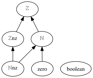
ℤ: integers
ℤnz: non-zero integers
ℕ: natural numbers
ℕnz: non-zero natural numbers
zero: the number 0

Operators:

ℤ + ℤ : ℤ
ℤ - ℤ : ℤ
ℤ × ℤ : ℤ
ℤ div ℤnz : ℤ (integer division)
ℤ rem ℤnz : ℤ (division remainder)
ℤℕnz : ℤ
ℤzero : ℕnz
abs(ℤ) : ℕ
ℤ < ℤ : boolean
ℤ ≤ ℤ : boolean
ℤ > ℤ : boolean
ℤ ≥ ℤ : boolean

4.2.3 Context "builtins/rational-numbers"

Includes "builtins/integers".

Sort graph:

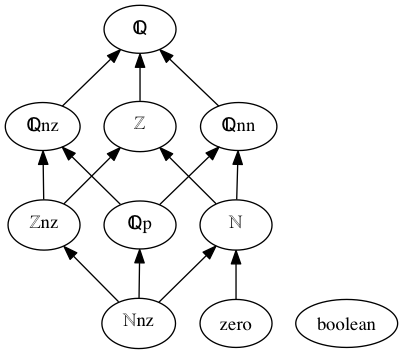
ℚ: rational numbers
ℚnz: non-zero rational numbers
ℚp: positive rational numbers
ℚnn: non-negative rational numbers

Operators:

ℚ + ℚ : ℚ
ℚ - ℚ : ℚ
ℚ × ℚ : ℚ
ℚ ÷ ℚnz : ℚ
ℚnzℤnz : ℚnz
ℚnzzero : ℕnz
abs(ℚ) : ℚnn
ℚ < ℚ : boolean
ℚ ≤ ℚ : boolean
ℚ > ℚ : boolean
ℚ ≥ ℚ : boolean

4.2.4 Context "builtins/real-numbers"

Includes "builtins/rational-numbers".

Sort graph:

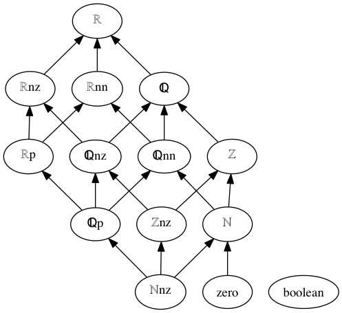
ℝ: real numbers
ℝnz: non-zero real numbers
ℝp: positive real numbers
ℝnn: non-negative real numbers

Operators:

ℝ + ℝ : ℝ
ℝ - ℝ : ℝ
ℝ × ℝ : ℝ
ℝ ÷ ℝnz : ℝ
ℝnzℤnz : ℝnz
ℝℕnz : ℝ
ℝpℝnz : ℝp
abs(ℝ) : ℝnn
√(ℝnn) : ℝnn
ℝ < ℝ : boolean
ℝ ≤ ℝ : boolean
ℝ > ℝ : boolean
ℝ ≥ ℝ : boolean

4.2.5 Context "builtins/IEEE-floating-point"

Includes "builtins/integers".

Sort graph:

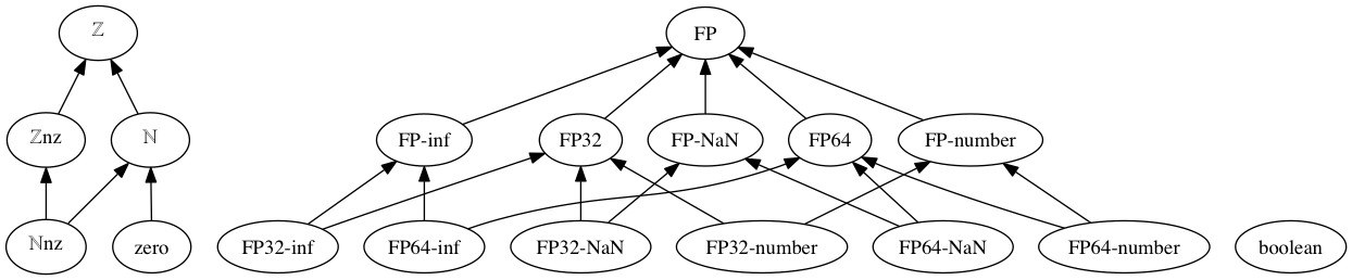
FP: any floating-point value
FP-number: floating-point number
FP-NaN: floating-point not-a-number
FP-inf: floating-point infinity
FP32: single-precision floating-point value
FP32-number: single-precision floating-point number
FP32-NaN: single-precision floating-point not-a-number
FP32-inf: single-precision floating-point infinity
FP64: double-precision floating-point value
FP64-number: double-precision floating-point number
FP64-NaN: double-precision floating-point not-a-number
FP64-inf: double-precision floating-point infinity

Operators:

FP32 + FP32 : FP32
FP64 + FP64 : FP64
FP32 - FP32 : FP32
FP64 - FP64 : FP64
FP32 × FP32 : FP32
FP64 × FP64 : FP64
FP32 ÷ FP32 : FP32
FP64 ÷ FP64 : FP64
FP32FP32 : FP32
FP64FP64 : FP64
abs(FP32) : FP32
abs(FP64) : FP64
√(FP32) : FP32
√(FP64) : FP64
FP32 < FP32 : boolean
FP64 < FP64 : boolean
FP32 ≤ FP32 : boolean
FP64 ≤ FP64 : boolean
FP32 > FP32 : boolean
FP64 > FP64 : boolean
FP32 ≥ FP32 : boolean
FP64 ≥ FP64 : boolean

1	What’s a digital scientific notation?
2	An overview of Leibniz
3	The anatomy of a Leibniz document
4	Leibniz reference